Documentation/How Tos/Calc: Derivation of Financial Formulas

Derivation of Financial Formulas

One factor that may hold back the use of Calc's Financial Functions is that of not understanding exactly how they are calculated. Some users may feel more comfortable knowing how the formulas have been derived, and this page is for them.

Most users will of course not wish to investigate further, and can ignore this page.

!! This page is currently in development !!

DB

This is a practical method. If the first year does not have 12 months, the total depreciation calculated is not exact; the method was originally useful because it is fairly easy to work out manually.

We wish to find a constant rate r, which when applied to the asset’s book value each year will give depreciation which reduces the asset’s value from c, the original cost, to s, the salvage value. We will assume the first year has 12 months, and the depreciation period (lifetime) is t years.

In the first year

Starting book value = c

Depreciation = cr

Remaining book value = c(1 - r)

In the second year

Starting book value = c(1 - r)

Depreciation = c(1 - r)r

Remaining book value = c(1 - r)(1 - r)

=c(1 - r)²

In the tth year

Final remaining book value = c(1 - r)^t

So

s = c(1 - r)^t

(s/c)^1/t = (1 - r)

r = 1 - (s/c)^1/t

The method is exact with whole years, but will slightly underestimate total depreciation if the first year has less than 12 months.

DDB

As with DB, the book value at the end of life is:

c(1 - r)^t

or the salvage value s if that is greater, where by definition: r = f/t (factor f and lifetime t).

The circumstances in which DDB will not depreciate to the salvage value are therefore:

s < c(1 - r)^t

=>

s / c < (1 - f/t)^t

SYD

With a depreciation period (lifetime) of t years, we'll find the depreciation in the y^th year:

Depreciation reduces the asset’s value from c, the original cost, to s, the salvage value, so the loss of value is c - s.

The sum of the years' digits is 1 + 2 + ... t = t(t+1)/2 (a standard result).

The years taken backward are t, t-1, .... 2, 1, which is (t+1 - y).

The depreciation in year y is therefore

(c - s) * (t+1 - y) / [ t(t+1)/2 ]

= (c - s) * (t+1 - y) * 2/ [t(t+1)]

Time Value of Money

Present and future values

We can invest $100 at say 5% annual interest, and in a year's time it is worth $105. Thus money in the hand today is worth more than the same money given to us later, because if we have money today, we can invest it and get interest on it.

The value of an investment today is called the 'present value'. The value of an investment at some time in the future is called the 'future value'. In this simple example the present value is $100 and the future value $105, if you assume an interest rate of 5%.

The choice of interest rate when calculating present and future values is important. It is often a choice that you make - and gives a present or future value to you, based on that rate. The rate is sometimes called the 'required rate of return'.

We will calculate a future value f of a sum p that we have today. Let us say there is an alternative investment with a rate r which compounds annually (that is, at the end of each year the interest is calculated and added to the investment), and we choose to use this rate.

At first our investment is worth p.

At the end of the 1st year it is worth p plus a year's interest

= p + pr = p(1 + r).

At the end of the 2nd year it is worth p(1 + r) plus a year's interest

= p(1 + r) + p(1 + r)r = p(1 + r)².

...

At the end of the nth year it is worth p(1 + r)ⁿ.

So the future value after n years is:

f = p(1 + r)ⁿ.

The present value is therefore:

p = f / (1 + r)ⁿ.

We have considered annually compounded interest, but this formula applies to any period (months, quarters, etc) where the interest rate (r per period) is compounded each period.

Make sure that you understand the difference between compounded and un-compounded interest. A rate of 1% per month uncompounded on an investment of $100 simply gives $1 per month - $12 interest in a year. A rate of 1% per month, compounded monthly, gives 100*(1*0.01)¹²-100 = $12.68 in the first year, and more in the second year.

Also note that this model assumes that the rate stays the same.

EFFECTIVE; EFFECT_ADD; (EFFECT); NOMINAL; NOMINAL_ADD

An investment is currently worth p, and pays interest at a rate of r each period, compounded.

From above, at the end of the nth period, the value of the investment = p(1 + r)ⁿ.

If the investment has a nominal rate x, say per year, and pays n times during each year, the interest rate paid each period ( 1/n th of a year ) is r = x/n.

As the interest compounds each period, the value of the investment at the end of the (say) year will be:

p(1 + r)ⁿ = p(1 + x/n)ⁿ.

We're looking for an effective rate e that would increase the value to the same amount as a result of one single interest payment.

p(1 + e) = p(1 + x/n)ⁿ

therefore

e = (1 + x/n)ⁿ - 1

and

x = n((1 + e)^1/n - 1)

Loans and Annuities

We will use a general model to describe both loans and annuities, where we borrow or invest a sum, we make or receive a number of regular payments, and at the end we pay or receive a final sum. Sometimes only two of these sums are needed - for example with a loan we might borrow the initial sum and then make monthly payments (there being no final sum). We define:

p = present value (the sum borrowed or invested)

f = future value (the sum to pay or be paid after n periods)

m = payment each period (does not change)

n = number of periods (a period may be a month, a year or whatever)

r = interest rate (fixed rate) per period (whatever length that is)

In the model, interest is calculated and applied to the balance each period.

We'll use a convention that a positive sum is money that we receive, and a negative sum is money that we pay. Thus if we take out a loan of $1000, paying regular instalments of $50, p is +$1000 and m is -$50; if we buy an annuity for $6000 which pays $30 regularly, p is -$6000 and m is +$30.

The sum of the future values (at the end of the term) of the cash flows will be zero. For example, I pay $100 into an account at 5% interest (p=-100). The future value of this (1 year in the future) is -105; the sum I withdraw from the account after 1 year is $105 (f=+105). The sum of future values is -105 + +105 which is zero.

The three cash flows are: the initial sum p, the periodic payments m and the final sum f.

The future value of p is p(1+r)ⁿ (see Present and Future Values, above).

There are n payments of m:

·When payments are made at the end of each period, the future value of the last payment will be m (it arises on the final date); the future value of the payment before that will be m(1+r)... ; the future value of the first payment will be m(1+r)^n-1. Summing those future values we get m[1 + (1+r) + (1+r)^{2 .....} (1+r)^n-1] = m[(1-(1+r)ⁿ)/(1-(1+r))] = m[(1-(1+r)ⁿ)/(-r)] = m[((1+r)ⁿ-1)/r], using standard result for a geometric series that 1+ a + a² .... a^n-1 = (1+aⁿ)/(1-a).

·When payments are made at the start of each period, the future value of the last payment will be m(1+r)... ; the future value of the first payment will be m(1+r)ⁿ. Summing those future values we get m[((1+r)ⁿ-1)/r](1+r).

·Combining these, where t is the type of payment: t=0 for end of period, t=1 for start of period, the future value of the payments is m[((1+r)ⁿ-1)/r](1+rt).

The future value of f is simply f, as it actually arises on our future date.

The equation for the sum of the 3 cash flows is therefore:

p(1+r)ⁿ + m[((1+r)ⁿ-1)/r](1+rt) + f = 0

PV, FV, PMT, NPER, RATE

These functions solve the annuity equation given above

p(1+r)ⁿ + m[((1+r)ⁿ-1)/r](1+rt) + f = 0

So:

PV: p = (-m[((1+r)ⁿ-1)/r](1+rt) - f) / (1+r)ⁿ

FV: f = -p(1+r)ⁿ - m[((1+r)ⁿ-1)/r](1+rt)

PMT: m = (-p(1+r)ⁿ - f) / [[((1+r)ⁿ-1)/r](1+rt)] = (-p(1+r)ⁿ - f)r / [((1+r)ⁿ-1)(1+rt)]

NPER: re-arrange the equation and take logs

RATE: the equation is solved by iteration - there is no general theoretical alternative.

IMPT, PPMT

These calculate how much of each payment is interest (IPMT) and how much is repaid capital (PPMT). PPMT is simply the payment (PMT) less the interest (IPMT), so our task here is to calculate that interest.

The interest included in a payment is the outstanding balance at the start of the preceding period times the interest rate. Here the 'preceding period' is the period before the payment is made - that is, the current period if the payment is made at the end of the period, or the period before that if the payment is made at the start of the period.

We will now derive the relevant outstanding balances.

The annuity equation we found earlier expresses future values at the end of term, that is, at the end of period n. We will apply that equation to preceding periods.

For payments made at the end of the period (t=0), going back one period simply removes one payment. For period x we have

p(1+r)^x + m[((1+r)^x-1)/r](1+rt) + f_x = 0

or

p(1+r)^x + m((1+r)^x-1)/r + f_x = 0

f_x is the outstanding balance at that time - that is the end of period x; we require the outstanding balance at the start of the period, that is f_x-1 given by:

p(1+r)^x-1 + m((1+r)^x-1-1)/r + f_x-1 = 0

The interest is given by rf_x-1, that is:

-rp(1+r)^x-1 - m((1+r)^x-1-1).

For payments made at the start of the period (t=1), for the time up to and including period x (< n) there is a payment at the very start of the term, followed by x payments at the end of the periods. We can use the annuity equation with an initial value of p + m (instead of p), where payments are made at the end:

(p+m)(1+r)^x + m((1+r)^x-1)/r + f_x = 0

This gives us the value (outstanding balance) at the end of period x. In fact the payment is made at the start of the period, and is calculated on the balance at the start of the period before that; that balance is therefore given by f_x-2, where:

(p+m)(1+r)^x-2 + m((1+r)^x-2-1)/r + f_x-2 = 0

and the interest is given by rf_x-2, that is:

-r(p+m)(1+r)^x-2 - m((1+r)^x-2-1).

ISPMT

We take out a loan. We will pay the capital off in fixed instalments every period. Each period we will also pay the interest due on the outstanding capital. The first instalment is at the start of the term. The last instalment is at the start of the last period.

n = number of periods (a period may be a month, a year or whatever)

p = principal (the capital sum borrowed)

r = interest rate (fixed rate) per period (not necessarily per month or year)

Repayment of capital each period (does not change) = p/n

At start of 1st period:

Capital outstanding = p - p/n = p(n-1)/n

Interest for the period = (p(n-1)/n) r

At start of 2nd period:

Capital outstanding = p(n-1)/n - p/n = p(n-2)/n

Interest for the period = (p(n-2)/n) r

At the start of the xth period:

Capital outstanding = p(n-x)/n

Interest for the period = (p(n-x)/n) r

=pr(n-x)/n

INTRATE

(to be written)

PRICE

PRICE returns:

present_value_of_coupon_payments + present_value_of_redemption_payment - accrued_coupon_interest.

The present value of the redemption payment is calculated as:

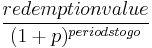
where redemptionvalue is the redemption payment, p is the yield per coupon period (= yield/frequency) and periodstogo is the (possibly fractional) number of periods remaining after the settlement date.

periodstogo is calculated as: number of whole periods + (number of days from settlement to the next coupon / number of days in the period containing the settlement date).

This appears to be a conventional way to calculate present value for partial periods, but it is worth noting that it could be seen as an estimate rather than exact. For example, $100 invested for a year at 10% yields (a 'redemption payment' of) $110. The present value of $110 halfway through the year calculates as 110/1.1^0.5 which is $104.88, yet we'd expect to get $105 for half a year at 10%.

The present value of the coupon payments is calculated as:

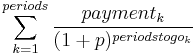
where payment is the coupon payment per $100 face value = 100*rate/frequency, periods is the number of whole periods remaining after settlement, periodstogo_k is the (possibly fractional) number of periods from settlement to that payment.

The accrued coupon interest is calculated per $100 face value as

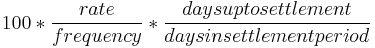
where daysuptosettlement is the number of days from the payment date just before settlement, and daysinsettlementperiod is the number of days in the period containing the settlement date.

'Number of days' is calculated throughout according to the calendar system ('basis') in use - see Financial date systems.

PRICEDISC

PRICEDISC returns:

redemptionvalue - (redemptionvalue * discountrate * days_to_maturity / days_in_year).

In other words the discounted amount is calculated proportionately and simply subtracted from the redemption value.

In basis 1, the definition of 'number of days in a year' is unclear - it may be 365 or 366, or (in Excel) somewhere in between. See Financial date systems.

PRICEMAT

PRICEMAT returns:

present_value_of_redemptionvalue_and_interest - accrued_interest

Values are per 100, so the redemption capital value is simply 100.

The interest paid at redemption is 100 * rate * days_in_issue / days_in_year. The fraction days_in_issue / days_in_year is calculated using YEARFRAC(issuedate; maturitydate; basis) in Calc. Excel does not specify its method of calculation.

The sum paid at redemption is therefore:

100 + 100 * rate * YEARFRAC(issuedate; maturitydate; basis)

The present value of that sum is calculated as:

(100 + 100 * rate * YEARFRAC(issuedate; maturitydate; basis)) / (1 + yield * YEARFRAC(settlementdate; maturitydate; basis)).

This takes no account of compounding. For example the present value of $150 received 5 years hence using a yield of 10% is calculated as 150/(1+0.1*5) = $100; with compounding that would be 150/(1+0.1)^5 = $93.14 approximately. It is important to understand this.

The accrued interest is calculated as 100 * rate * days_before_settlement / days_in_year, that is:

100 * rate * YEARFRAC(issuedate; settlementdate; basis)).

Note that there are known issues with YEARFRAC (the length of a year in basis 1; basis 0 date adjustments) that affect both Excel and Calc.

This may be a standard method of calculation in the US. Its validity elsewhere is uncertain. The entire formula is :

[(100 + 100 * rate * YEARFRAC(issuedate; maturitydate; basis)) / (1 + yield * YEARFRAC(settlementdate; maturitydate; basis))] - 100 * rate * YEARFRAC(issuedate; settlementdate; basis)).

YIELD

We saw above that PRICE returns:

present_value_of_coupon_payments + present_value_of_redemption_payment - accrued_coupon_interest

which is:

where p is the yield per coupon period (= yield/frequency).

There is no general way to re-arrange this equation to solve for yield. Thus a starting guess for yield is chosen, and then repeatedly adjusted to bring the calculated value of PRICE close to the value specified as a parameter in the YIELD function.

YIELDMAT

The bond pays interest just once, at maturity. The yield is calculated from this straightforward formula:

maturity _value / settlement_value = 1 + yield*YEARFRAC(settlement;maturity),

where YEARFRAC(settlement;maturity) is the fraction: number_of_days_between_settlement_and_maturity divided by the number_of_days_in_a_year.

Now:

maturity _value = redemption_value + interest

= 100 + 100*rate*YEARFRAC(issue;maturity)

= 100*(1+rate*YEARFRAC(issue;maturity))

where rate is the annual interest rate.

settlement_value can be found from the equation for PRICEMAT:

price = presentvalue_of_redemption_and_interest - accrued_interest

= settlement_value - accrued_interest

=> settlement_value = price + accrued_interest

= price + 100*rate*YEARFRAC(issue;settlement)

From above:

1 + yield*YEARFRAC(settlement;maturity) = maturity _value / settlement_value

=> yield = (maturity _value / settlement_value - 1)/YEARFRAC(settlement;maturity)

= (100*(1+rate*YEARFRAC(issue;maturity)) / (price + 100*rate*YEARFRAC(issue;settlement)) - 1)/YEARFRAC(settlement;maturity)

where all the YEARFRACs are calculated using the correct basis.

See also:

Financial date systems

Financial functions