Documentation/OOoAuthors User Manual/Getting Started/Getting Started with Calc

Template:NeedsWork This page was created by converting ODT to Mediawiki using Writer2MediaWiki.

This is Chapter 7 of Getting Started with OpenOffice.org 2.x (Third edition), produced by the OOoAuthors group. A PDF of this chapter is available from the OOoAuthors Guides page at OpenOffice.org.

<< User Manuals page
<< Getting Started Table of Contents
<< Chapter 6 Getting Started with Writer   |   Chapter 8 Getting Started with Draw >>

What is Calc?

Calc is the spreadsheet component of OpenOffice.org (OOo). You can enter data, usually numerical data, in a spreadsheet and then manipulate this data to produce certain results.

Alternatively you can enter data and then use Calc in a 'What If...' manner by changing some of the data and observing the results without having to retype the entire spreadsheet or sheet.

Spreadsheets, sheets, and cells

Calc works with elements called spreadsheets. Spreadsheets consist of a number of individual sheets, each containing a block of cells arranged in rows and columns.

These cells hold the individual elements—text, numbers, formulas etc., which make up the data to be displayed and manipulated.

Each spreadsheet can have many sheets and each sheet can have many individual cells. Each sheet in Calc can have a maximum of 65,536 rows and a maximum of 245 columns (A through IV). This gives 16,056,320 individual cells per sheet.

Parts of the main Calc window

When Calc is started, the main window looks similar to Figure 1.

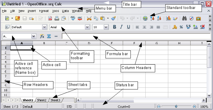
Figure 1: Parts of the Calc window.

Formula bar

On the left of the Formula bar (see Figure 2) is a small text box, called the Name box, with a letter and number combination in it, such as D7. This is the column letter and row number, called the cell reference, of the current cell.

Figure 2. Formula Bar.

To the right of the Name box are the Function Wizard, Sum, and Function buttons.

Clicking the Function Wizard button opens a dialog from which you can search through a list of available functions. This can be very useful, because it also shows how the functions are formatted.

The Sum button inserts a formula into the current cell that totals the numbers in the cells above, or to the left if there are no numbers above, the current cell.

The Function button inserts an equals sign into the selected cell and the Input Line, thereby setting the cell ready to accept a formula.

When you enter data into a cell, the Sum and Equals buttons change to Cancel and Accept buttons.

The contents of the current cell (data, formula, or function) are displayed in the Input Line, the remainder of the Formula bar. You can edit the cell contents of the current cell in the Input Line, or you can do that in the current cell. To edit inside the Input Line area, left-click the appropriate part of the Input Line area, then type your changes. To edit within the current cell, double-click the cell.

Individual cells

The main section of the screen displays the individual cells in the form of a grid, with each cell being at the intersection of a particular column and row.

At the top of the columns and at the left-hand end of the rows are a series of gray boxes containing letters and numbers. These are the column and row headers. The columns start at A and go on to the right and the rows start at 1 and go on down.

Sheet tabs

At the bottom of the grid of cells are the sheet tabs (see Figure 3). These tabs enable access to each individual sheet, with the visible, or active, sheet having a white tab.

Clicking on another sheet tab displays that sheet and its tab turns white. You can also select multiple sheet tabs at once by holding down the Control key while you click the names.

Figure 3. Sheet tabs.

File management

Starting new spreadsheets

A new spreadsheet can be opened regardless of which other component of OOo you are using at the time. For example, a new spreadsheet can be opened from Writer or Draw.

• From the menu bar—Click File and then select New > Spreadsheet.
• From the toolbar—Use the New Document button on the Standard toolbar. Click the drop-down arrow for a choice of what type of document to open (text document, spreadsheet, and so on). Click the button itself to create a new document of the type that is currently open (if a spreadsheet is open, a new spreadsheet document will be created).
• From the keyboard—If you already have a spreadsheet open, you can press Control+N to open a new spreadsheet.

Opening existing spreadsheets

A spreadsheet can also be opened no matter what component of OOo you are in.

• From the menu bar—Click File and then select Open.
• From the toolbar—Click the Open button on the Standard toolbar.
• From the keyboard—Use the key combination Control+O.

Each of these options displays the Open dialog, where you can locate the spreadsheet that you want to open.

Saving spreadsheets

Spreadsheets can be saved in three ways.

• From the menu bar—Click File and then select Save.
• From the toolbar—Click on the Save button on the Function bar.
• From the keyboard—Use the key combination Control+S.

If the spreadsheet has not been saved previously, then each of these actions will open the Save As dialog. Here you can specify the spreadsheet name and the location in which to save the spreadsheet.

Navigating within spreadsheets

Going to a particular cell

Using the mouse

Place the mouse pointer over the cell and left-click.

Using a cell reference

Click on the little inverted black triangle just to the right of the Name box (Figure 2). The existing cell reference will be highlighted. Type the cell reference of the cell you want to go to and press Enter. Or just click into the Name box, backspace over the existing cell reference and type in the cell reference you want.

Using the Navigator

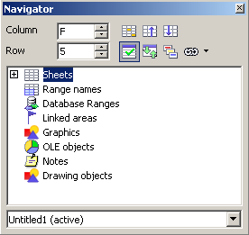
Click on the Navigator button in the Standard toolbar (or press F5) to display the Navigator. Type the cell reference into the top two fields, labeled Column and Row, and press Enter. In Figure 4 the Navigator would select cell F5.

Figure 4. Calc Navigator.

Moving from cell to cell

In the spreadsheet, one cell, or a group of cells, normally has a darker black border. This black border indicates where the focus is (see Figure 5).

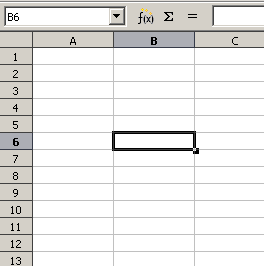
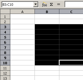
Figure 5. (Left) One selected cell and (right) a group of selected cells

Using the Tab and Enter keys

• Pressing Enter or Shift+Enter moves the focus down or up, respectively.
• Pressing Tab or Shift+Tab moves the focus right or left, respectively.

Using the cursor keys

Pressing the cursor keys on the keyboard moves the focus in the direction of the arrows.

Using Home, End, Page Up and Page Down

• Home moves the focus to the start of a row.
• End moves the focus to the column furthest to the right that contains data.
• Page Down moves the display down one complete screen and Page Up moves the display up one complete screen.
• Combinations of Control and Alt with Home, End, Page Down, Page Up, and the cursor keys move the focus of the current cell in other ways.

Tip: Holding down Alt+Cursor key resizes a cell.

Moving from sheet to sheet

Each sheet in a spreadsheet is independent of the others though they can be linked with references from one sheet to another. There are three ways to navigate between different sheets in a spreadsheet.

Using the keyboard

Pressing Control+PgDn moves one sheet to the right and pressing Control+PgUp moves one sheet to the left.

Using the mouse

Clicking one of the Sheet Tabs (see Figure 3) at the bottom of the spreadsheet selects that sheet.

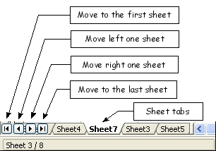
If you have a lot of sheets, then some of the sheet tabs may be hidden behind the horizontal scroll bar at the bottom of the screen. If this is the case, then the four buttons at the left of the sheet tabs can move the tabs into view. Figure 6 shows how to do this.

Figure 6. Sheet tab arrows

Notice that the sheets here are not numbered in order. Sheet numbering is arbitrary—you can name a sheet as you wish.

Note: The sheet tab arrows that appear in Figure 6 only appear if you have some sheet tabs that can not be seen. Otherwise they will appear faded as in Figure 3.

Selecting items in a sheet or spreadsheet

Selecting cells

Cells can be selected in a variety of combinations and quantities.

Single cell

Left-click in the cell. The result will look like the left side of Figure 5. You can verify your selection by looking in the Name box.

Range of contiguous cells

A range of cells can be selected using the keyboard or the mouse.

To select a range of cells by dragging the mouse:

1. Click in a cell.
2. Press and hold down the left mouse button.
3. Move the mouse around the screen.
4. Once the desired block of cells is highlighted, release the left mouse button.

To select a range of cells without dragging the mouse:

1. Click in the cell which is to be one corner of the range of cells.
2. Move the mouse to the opposite corner of the range of cells.
3. Hold down the Shift key and click.

To select a range of cells without using the mouse:

1. Select the cell that will be one of the corners in the range of cells.
2. While holding down the Shift key, use the cursor arrows to select the rest of the range.

The result of any of these methods will look like the right side of Figure 5.

Tip: You can also directly select a range of cells using the Name box. Click into the Name box as described in Using a cell reference. To select a range of cells, enter the cell reference for the upper left hand cell, followed by a colon (:), and then the lower right hand cell reference. For example, to select the range that would go from A3 to C6, you would enter A3:C6.

Range of non-contiguous cells

1. Select the cell or range of cells using one of the methods above.
2. Move the mouse pointer to the start of the next range or single cell.
3. Hold down the Control key and click or click-and-drag to select a range.
4. Repeat as necessary.

Selecting columns and rows

Entire columns and rows can be selected very quickly in OOo.

Single column or row

To select a single column, click on the column identifier letter (see Figure 1).

To select a single row, click on the row identifier number (see Figure 1).

Multiple columns or rows

To select multiple columns or rows that are contiguous:

1. Click on the first column or row in the group.
2. Hold down the Shift key.
3. Click the last column or row in the group.

To select multiple columns or rows that are not contiguous:

1. Click on the first column or row in the group.
2. Hold down the Control key.
3. Click on all of the subsequent columns or rows while holding down the Control key.

Entire sheet

To select the entire sheet, click on the small box between the A column header and the 1 row header (Figure 7). You can also use the keyboard to select the entire sheet by pressing Control+A.

Figure 7. Select All box.

Working with columns and rows

Inserting columns and rows

Columns and rows can be inserted in several different way and quantities.

Single column or row

A single column or row can be added using the Insert menu:

1. Select the column or rows where you want the new column or row inserted.
2. Select either Insert > Column or Insert > Row.

Note: When you insert a single new column, it is inserted to the left of the highlighted column. When you insert a single new row, it is inserted above the highlighted row.

A single column or row can also be added using the mouse:

1. Select the column or row where you want the new column or row inserted.
2. Right-click the header.
3. Select Insert Row or Insert Column.

Multiple columns or rows

Multiple columns or rows can be inserted at once rather than inserting them one at a time.

1. Highlight the required number of columns or rows by holding down the left mouse button on the first one and then dragging across the required number of identifiers.
2. Proceed as for inserting a single column or row above.

Deleting columns and rows

Columns and rows can be deleted individually or in groups.

Single column or row

A single column or row can only be deleted by using the mouse:

1. Select the column or row to be deleted.
2. Right-click on the column or row header.
3. Select Delete Column or Delete Row from the pop-up menu.

Multiple columns or rows

Multiple columns or rows can be deleted at once rather than deleting them one at a time.

1. Highlight the required number of columns or rows by holding down the left mouse button on the first one and then dragging across the required number of identifiers.
2. Proceed as for deleting a single column or row above.

Working with sheets

Like any other Calc element, sheets can be inserted, deleted and renamed.

Inserting new sheets

There are many ways to insert a new sheet. The first step for all of the methods is to select the sheets that the new sheet will be inserted next to. Then any of the following options can be used.

• Click on the Insert menu and select Sheet, or
• Right-click on its tab and select Insert Sheet, or
• Click into an empty space at the end of the line of sheet tabs (see Figure 8).

Figure 8. Inserting a new sheet

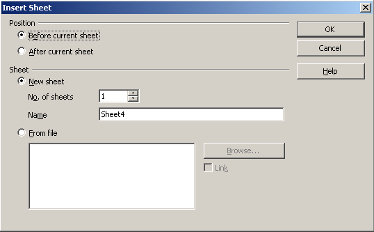
Each method will open the Insert Sheet dialog (Figure 9). Here you can select whether the new sheet is to go before or after the selected sheet and how many sheets you want to insert. If you are inserting only one sheet, there is the opportunity to give the sheet a name.

Figure 9. Insert Sheet dialog

Deleting sheets

Sheets can be deleted individually or in groups.

'Single 'sheet

Right-click on the tab of the sheet you want to delete and select Delete from the pop-up menu.

Multiple 'sheet's

To delete multiple sheets, select them as described earlier, right-click on one of the tabs and select Delete from the pop-up menu.

Renaming sheets

The default name for the a new sheet is "SheetX", where X is a number. While this works for a small spreadsheet with only a few sheets, it becomes awkward when there are many sheets.

To give a sheet a more meaningful name, you can:

• Enter the name in the name box when you create the sheet, or
• Right-click on a sheet tab and select Rename Sheet from the pop-up menu and replace the existing name with a better one.

Note: Sheet names must start with either a letter or a number; other characters including spaces are not allowed. Aside from the first character of the sheet name, allowed characters are letters, numbers, spaces, and the underline character. Attempting to rename a sheet with an invalid name will produce an error message.

Viewing Calc

Freezing rows and columns

Freezing locks a number of rows at the top of a sheet or a number of columns on the left of a sheet or both. Then when scrolling around within the sheet, any frozen columns and rows remain in view.

Figure 10 shows some frozen rows and columns. The heavier horizontal line between rows 3 and 14 and the heavier vertical line between columns C and H denote the frozen areas. Rows 4 through 13 and columns D through G have been scrolled off the page. Because the first three rows and columns are frozen into place, they remained.

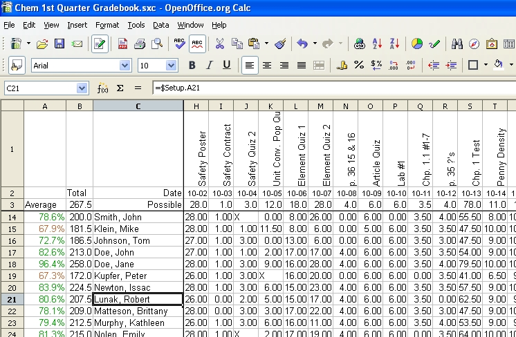
Figure 10. Frozen rows and columns.

You can set the freeze point at one row, one column, or both a row and a column as in Figure 10.

Freezing single rows or columns

1. Click on the header for the row below where you want the freeze or for the column to the right of where you want the freeze.
2. Select Window > Freeze.

A dark line will appear to indicate where the freeze is put.

Freezing a row and a column

1. Click into the cell that is immediately below the row you want frozen and immediately to the right of the column you want frozen.
2. Select Window > Freeze.

You will see two lines appear on the screen, a horizontal line above this cell and a vertical line to the left of this cell. Now as you scroll around the screen everything above and to the left of these lines will remain in view.

Unfreezing

To unfreeze rows or columns, select Window > Freeze. The checkmark by Freeze will vanish.

Splitting the window

Another way to change the view is by splitting the window—otherwise known as splitting the screen. The screen can be split either horizontally or vertically or both. This allows you to have up to four portions of the sheet in view at any one time.

Why would you want to do this? Imagine you have a large sheet and one of the cells has a number in it which is used by three formulas in other cells. Using the split screen technique, you can position the cell containing the number in one section and each of the cells with formulas in the other sections. Then you can change the number in the cell and watch how it affects each of the formulas.

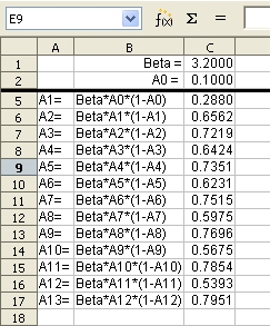
Figure 11. Split screen example.

Splitting the screen horizontally

To split the screen horizontally:

1. Move the mouse pointer into the vertical scroll bar, on the right-hand side of the screen, and place it over the small button at the top with the black triangle.
2. Immediately above this button you will see a thick black line (Figure 12). Move the mouse pointer over this line and it will turn into a line with two arrows.
3. Hold down the left mouse button and a grey line will appear, running across the page. Drag the mouse downwards and this line will follow.
4. Release the mouse button and the screen will split into two views, each with its own vertical scroll bar.

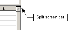
Figure 12. Split screen bar on vertical scroll bar.

Notice in Figure 11, the 'Beta' and the 'A0' values are in the upper part of the window and other calculations are in the lower part. You may scroll the upper and lower parts independently. Thus you can make changes to the Beta and A0 values and watch their affects on the calculations in the lower half of the window.

You can also split the window vertically as described below—with the same results, being able to scroll both parts of the window independently. With both horizontal and vertical splits, you have four independent windows to scroll.

Splitting the screen vertically

To split the screen vertically:

1. Move the mouse pointer into the horizontal scroll bar at the bottom of the screen and place it over the small button on the right with the black triangle.
2. Immediately to the right of this button you will see a thick black line (Figure 13). Move the mouse pointer over this line and it will turn into a line with two arrows.
3. Hold down the left mouse button and a grey line will appear, running up the page. Drag the mouse to the left and this line will follow.
4. Release the mouse button and the screen will be split into two views, each with its own horizontal scroll bar.

Figure 13: Split bar on horizontal scroll bar.

Note: Splitting the screen horizontally and vertically at the same time will give four views, each with its own vertical and horizontal scroll bars.

Removing split views

• Double-click on each split line, or
• Click on and drag the split lines back to their places at the ends of the scroll bars, or
• Select Window > Split. This will remove all split lines at the same time.

Tip: You can also split the screen using a menu command. Click in a cell that is immediately below and immediately to the right of where you wish the screen to be split, and choose Window > Split.

Entering data into a sheet

Entering numbers

Select the cell and type in the number using either the top row of the keyboard or the numeric keypad.

To enter a negative number, type a minus (–) sign in front of it or enclose it in brackets ( ).

By default numbers are right-aligned and negative numbers have a leading minus symbol.

Entering text

Select the cell and type the text. Text is left-aligned by default.

Entering numbers as text

If a number is entered in the format 01481, Calc will drop the leading 0. To preserve the leading zero, in the case of telephone area codes for example, precede the number with an apostrophe, like this: '01481. However, the data is now regarded as text by Calc. Formulas and functions will treat the entry like any other text entry, which typically results in it being a zero in a formula, and being ignored in a function.

Note: When entering an apostrophe to allow a leading zero to be displayed, the apostrophe will not be visible in the cell after the Enter key is pressed only if the apostrophe is a plain apostrophe (not a "smart quote" apostrophe). The type of apostrophe is selected by choosing Tools > Autocorrect > Custom Quotes. The selection of the apostrophe type will affect Calc and Writer. If "smart quotes" are selected for apostrophes, the apostrophe will remain visible in the cell after pressing Enter.

Tip: Numbers can have leading zeros and be regarded as numbers (as opposed to text) if the cell is formatted appropriately. Right-click on the cell and choose Format Cells > Numbers. Adjust the leading zeros setting to add leading zeros to numbers.

Entering dates and times

Select the cell and type the date or time. You can separate the date elements with a slant (/) or a hyphen (-) or use text such as 10 Oct 03. Calc recognizes a variety of date formats. You can separate time elements with colons such as 10:43:45.

Printing

Calc offers a powerful and highly configurable printing system. Many different details can be selected to print or not to print. The order the sheets will print in can be specified, as well as their size. Particular rows or columns can be specified to print on all sheets and the print range can be specified.

Printing a spreadsheet

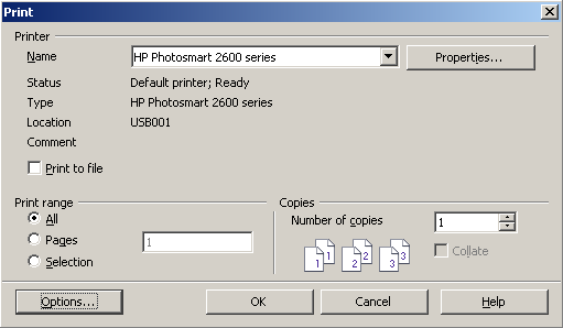
To print a spreadsheet either to a printer or a file, choose File > Print. The Print dialog (Figure 14) allows printer settings to be changed. What to print can be set quickly here: the whole document, specific sheets or a group of selected cells. The number of copies, and whether to collate the copies, are also set in this dialog. Choose OK to start printing.

Figure 14. The Print dialog.

Print options

Printer options can be set for the current document only or for all spreadsheets. To select for the current document, on the Print dialog, click the Options button in the bottom left. To set print options permanently, go to Tools > Options > OpenOffice.org Calc > Print. The dialog boxes for both are very similar. See Figure 15.

Figure 15. Print Options dialog.

Selecting sheets to print

One or more sheets can be selected for printing. This can be useful if you have a large spreadsheet with multiple sheets and only want a certain sheet to print. An example would be an accountant recording costs over time where there was one sheet for each month. If only the November sheet were to be printed, this is the procedure to follow.

1. Select the November sheet. (If more than one sheet is to be printed, hold down the Control key as you click on each sheet tab.)
2. Choose File > Print and select Options.

Note: The Options button is different from the Properties button. Properties deals with the settings of the printer, whereas Options deals with OOo's settings.

1. Check the Print only selected sheets checkbox. Click OK.

Adjusting the print range

Printing rows or columns on every page

If a sheet will be printed on multiple pages, certain rows or columns can be set up to repeat on each printed page.

As an example, if the top two rows of the sheet as well as column A need to be printed on all pages, do the following:

1. 1. Choose Format > Print Ranges > Edit Print Range.
   2. The Edit Print Ranges dialog (Figure 16) appears. Click on - none - to the left of the Rows to repeat area, and change it to - user defined -.
   3. In the text entry box in the center, type in the rows to repeat. For example, to repeat rows one and two, type $1:$2. (Or alternatively, click in cell A1 and drag to cell A2.)
   4. Columns can also repeat; click on - none - to the left of the Columns to repeat area, and change it to - user defined -.
   5. In the text entry box in the center, type in the columns to repeat. For example, to repeat column A, type $A. (Or alternatively, click in cell A1.)
   6. Click OK.

inline:Frame22.png

Note

The entire range of the rows to be repeated does not need to be selected. Just selecting one cell in each row will work.

Defining a print range

By default, if no print range has been defined, the entire contents of the worksheet will be printed. Optionally, a print range can be defined. Use this option to modify or set a defined print range. This could be useful if, in a large spreadsheet, only a specific area of data needs to be printed.

To define a print range:

1. 1. Highlight the range of cells that comprise the print range.
   2. Choose Format > Print Ranges > Define Print Range.

The page break lines will display on screen.

Note

You can check the print range by using File > Page Preview. OOo will only display the cells in the print range.

Adding to the print range

After defining a print range, you can add more cells to it. This allows you to print multiple, non-contiguous areas of the same sheet, while not printing the whole sheet. Once you have defined a print range:

1. 1. Highlight the range of cells that should be added to the print range.
   2. Choose Format > Print Ranges > Add Print Range.

This will add the extra cells to the print range.

The page break lines will no longer show up on the screen.

Note

The additional print range will print as a separate page, even if both ranges are on the same sheet.

Removing a print range

It may become necessary to remove a defined print range, for example if the whole sheet needs to be printed at a later time.

To remove the print range, choose Format > Print Ranges > Clear Print Range.

This will remove all defined print ranges on the sheet.

After the print range is removed, the default page break lines will appear on the screen.